Detailed Input
The xcontrol instruction set is inspired by the Turbomole control
file syntax. I decided to call it xcontrol instructions back than,
but here we will just call it (detailed) input for convenience.
The man page can be found here.
Note
The parser implemented is more general and limited by arbitrary choice to this syntax. At some point more common formats like JSON, YAML or XML might become available as alternative input formats.
To read an input file called xtb.inp use
> xtb --input xtb.inp coord
In the detailed input you have control about almost every global variable in the program, some instructions even check your input, but most of the time you should know what you are doing. Developed as a feature for developers, this is incredible powerful and naturally way to complicated for the average application. So in most cases you can safely rely on the internal defaults or the shipped global configuration file (should usually be the same).
I will walk you through some selected instructions you might find useful for your application.
Fixing, Constraining and Confining
In xtb different concepts of constraints are implemented,
so you should know which tool is best for you problem before you
start writing the detailed input.
We will go through this sections using the caffeine molecule
24

C          1.07317        0.04885       -0.07573
N          2.51365        0.01256       -0.07580
C          3.35199        1.09592       -0.07533
N          4.61898        0.73028       -0.07549
C          4.57907       -0.63144       -0.07531
C          3.30131       -1.10256       -0.07524
C          2.98068       -2.48687       -0.07377
O          1.82530       -2.90038       -0.07577
N          4.11440       -3.30433       -0.06936
C          5.45174       -2.85618       -0.07235
O          6.38934       -3.65965       -0.07232
N          5.66240       -1.47682       -0.07487
C          7.00947       -0.93648       -0.07524
C          3.92063       -4.74093       -0.06158
H          0.73398        1.08786       -0.07503
H          0.71239       -0.45698        0.82335
H          0.71240       -0.45580       -0.97549
H          2.99301        2.11762       -0.07478
H          7.76531       -1.72634       -0.07591
H          7.14864       -0.32182        0.81969
H          7.14802       -0.32076       -0.96953
H          2.86501       -5.02316       -0.05833
H          4.40233       -5.15920        0.82837
H          4.40017       -5.16929       -0.94780
Exact Fixing
In the exact fixing approach the Cartesian position of the selected atom is fixed in space by setting its gradient to zero and the degrees of freedom are removed from the optimization procedure and therefore the atoms stay in place in geometry optimizations.
For dynamics this exact fixing is automatically deactivated, since it usually leads to instabilities in the simulation.
To activate the exact fixing for atoms 1–10 and atom 12 as well as for all oxygen atoms, add
$fix
   atoms: 1-10,12
   elements: O
$end
to your detailed input, the atoms keyword refers to the numbering of the individual atoms in your input geometry. With this input the verbose output will show a short summary of the fixed atoms:
           -------------------------------------------------
          |                   Fixed Atoms                   |
           -------------------------------------------------

 * 13 fixed atom positions, i.e. in gradient

     #   Z                                   position/Å
     1   6 C      1.0731700     0.0488500    -0.0757300
     2   7 N      2.5136500     0.0125600    -0.0758000
     3   6 C      3.3519900     1.0959200    -0.0753300
     4   7 N      4.6189800     0.7302800    -0.0754900
     5   6 C      4.5790700    -0.6314400    -0.0753100
     6   6 C      3.3013100    -1.1025600    -0.0752400
     7   6 C      2.9806800    -2.4868700    -0.0737700
     8   8 O      1.8253000    -2.9003800    -0.0757700
     9   7 N      4.1144000    -3.3043300    -0.0693600
    10   6 C      5.4517400    -2.8561800    -0.0723500
    12   7 N      5.6624000    -1.4768200    -0.0748700
     8   8 O      1.8253000    -2.9003800    -0.0757700
    11   8 O      6.3893400    -3.6596500    -0.0723200
Note
Since version 6.3 the input is sorted and duplicates are removed automatically.
Constraining Potentials
Almost absolute control about anything in your system is archived
by applying constraining potentials. First of all the constraining
potentials offer a weaker version of the exact fixing, which is
invoked by the same syntax in the $constrain data group as
$constrain
   atoms: 11
   elements: C,N,8
$end
the program will not attempt to hold the Cartesian positions constant, but the distances between all selected atoms, here number 11 and all carbon, nitrogen and oxygen. For each atom pair a harmonic potential is generated to hold the distances at roughly the starting value, this even works without problems in dynamics.
For your caffeine molecule this results in a problem, which can easily be spotted in the verbose output of the constraints summary.
           -------------------------------------------------
          |                   Constraints                   |
           -------------------------------------------------

 * 15 constrained atom positions
   positions referring to input geometry

     #   Z                                   position/Å      displ./Å
    11   8 O      6.3577347    -3.6327225    -0.0684681     0.0000000
     1   6 C      1.0687445     0.0520162    -0.0755782     0.0000000
     3   6 C      3.3535252     1.0744217    -0.0774722     0.0000000
     5   6 C      4.5969189    -0.6303196    -0.0745855     0.0000000
     6   6 C      3.2896462    -1.0950551    -0.0735452     0.0000000
     7   6 C      2.9629004    -2.4886091    -0.0702591     0.0000000
    10   6 C      5.4425717    -2.8389078    -0.0699228     0.0000000
    13   6 C      7.0086271    -0.9538835    -0.0749134     0.0000000
    14   6 C      3.9536622    -4.7147069    -0.0641970     0.0000000
     2   7 N      2.5030143     0.0336686    -0.0754494     0.0000000
     4   7 N      4.6213728     0.7205067    -0.0770658     0.0000000
     9   7 N      4.1215924    -3.2704219    -0.0683024     0.0000000
    12   7 N      5.6601563    -1.4769082    -0.0732293     0.0000000
     8   8 O      1.8493654    -2.9780046    -0.0690630     0.0000000
    11   8 O      6.3577347    -3.6327225    -0.0684681     0.0000000

     applying 105 atom pairwise harmonic potentials
       applied force constant per pair:     0.0035714
     effective force constant per atom:     0.0500000
         constraining energy/grad norm:     0.0000000     0.0000000
Note
Since version 6.3 the input is sorted and duplicates are removed automatically.
Note that in some versions of xtb this leads to NaN for the
gradient, therefore double-check the constrained atom list for duplicates.
To constrain the atoms more tightly the force constant can be adjusted
$constrain
   force constant=1.0
$end
this variable goes directly into the constraining procedure and is given in atomic unites (Hartree/Bohr²), for very high force constants this becomes equivalent to the exact fixing. Note the difference in the syntax as you are required to use an equal-sign instead of a colon, as you are modifying a global variable.
It is also possible to constrain selected internal coordinates, possible are distances, angles and dihedral angles as done here
$constrain
   distance: 1, 2, 1.4
   angle: 5, 7, 8, auto
   dihedral: 3, 4, 1, 7, 180
$end
Note
This printout is not yet fully integrated in the released versions and
might not work as expected.
For the experimental constraining potentials supporting this features
use the all-caps keyword variants (DISTANCE, ANGLE and DIHEDRAL).
Note that those are not available for the scan feature.
Distance constraints are given in Ångström, while angle constraints are given
in degrees.
The distances are defined by two atom number referring to the order in
your coordinate input, angles are defined by three atom numbers and
dihedral angles by four atoms, in any case the atoms do not have to
be connected by bonds. The last argument is always the value which should
be used in the constraining potential as reference, if you decide to
use the current value auto can be passed. The constraints will be
printed to the screen (the newer implementation may require the verbose mode,
to trigger the printout of the constraint summary), we check this setup
for the caffeine molecule
           -------------------------------------------------
          |                   Constraints                   |
           -------------------------------------------------

 * 1 constrained distance

     #   Z        #   Z                                     value/Å      actual/Å
     1   6 C      2   7 N                                 1.4000000     1.4409371

       constraining potential exponent:     2.0000000
      applied force constant per dist.:     0.0500000
     effective force constant per atom:     0.0250000
         constraining energy/grad norm:     0.0002992     0.0109403

 * 1 constrained angle

     #   Z        #   Z        #   Z                        value/°      actual/°
     5   6 C      7   6 C      8   8 O                  150.4357763   150.4357763

      applied force constant per angle:     0.0500000
     effective force constant per atom:     0.0166667
         constraining energy/grad norm:     0.0000000     0.0000000

 * 1 constrained dihedral angle

     #   Z        #   Z        #   Z        #   Z           value/°      actual/°
     3   6 C      4   7 N      1   6 C      7   6 C     180.0000000  -179.9396548

      applied force constant per angle:     0.0500000
     effective force constant per atom:     0.0125000
         constraining energy/grad norm:     0.0000000     0.0000629

     total constraint energy/grad norm:     0.0002993     0.0110032
You can find the constraint energy and gradient at the end of the summary, check for unphysical high values of the energy and gradient here to verify your constraint setup otherwise you might encounter strange behaviour in the following optimization or dynamics to adhere this constraints.
If you are not quite sure which distances or angles you want to constrain, run
> cat geosum.inp
$write
   distances=true
   angles=true
   torsions=true
$end
> xtb --define --verbose --input geosum.inp caffeine.xyz
and have a look at the geometry summary for your molecule. The $write
data group toggles the printout in the property section and also some
printouts in the input section.
For caffeine the geometry summary including only the distances looks like this
           -------------------------------------------------
          |                Geometry Summary                 |
           -------------------------------------------------

      molecular mass/u    :      194.1926000
   center of mass at/Å    :        4.0569420      -1.6298957      -0.0733327
  moments of inertia/u·Å² :        4.7317175E+02   7.1109348E+02   1.1745947E+03
rotational constants/cm⁻¹ :        3.5626878E-02   2.3706633E-02   1.4351872E-02

 * 25 selected distances

     #   Z        #   Z                                     value/Å
     1   6 C      2   7 N                                 1.4409371
     2   7 N      3   6 C                                 1.3698478
     3   6 C      4   7 N                                 1.3186949
     4   7 N      5   6 C                                 1.3623047
     2   7 N      6   6 C                                 1.3652477
     5   6 C      6   6 C                                 1.3618461
     6   6 C      7   6 C                                 1.4209574
     7   6 C      8   8 O                                 1.2271501
     7   6 C      9   7 N                                 1.3977057
     9   7 N     10   6 C                                 1.4104346
    10   6 C     11   8 O                                 1.2347703
     5   6 C     12   7 N                                 1.3741439
    10   6 C     12   7 N                                 1.3953559
    12   7 N     13   6 C                                 1.4514011 (max)
     9   7 N     14   6 C                                 1.4496299
     1   6 C     15   1 H                                 1.0929740
     1   6 C     16   1 H                                 1.0928728
     1   6 C     17   1 H                                 1.0928837
     3   6 C     18   1 H                                 1.0829302 (min)
    13   6 C     19   1 H                                 1.0932399
    13   6 C     20   1 H                                 1.0945661
    13   6 C     21   1 H                                 1.0945601
    14   6 C     22   1 H                                 1.0927021
    14   6 C     23   1 H                                 1.0949866
    14   6 C     24   1 H                                 1.0949141

 * 4 distinct bonds (by element types)

   Z      Z             #   av. dist./Å        max./Å        min./Å
   1 H    6 C          10     1.0926630     1.0949866     1.0829302
   6 C    6 C           2     1.3914017     1.4209574     1.3618461
   6 C    7 N          11     1.3941548     1.4514011     1.3186949
   6 C    8 O           2     1.2309602     1.2347703     1.2271501
There is no electronic structure information used at this point but a simple geometric model to select distances, which can get too few or too many bonds or angles in this printout.
Confining in a Cavity
If you are running dynamics for systems that are non-covalently bound, you may encounter dissociation in the dynamics. If you want to study the bound complex, you can try to confine the simulation in a little sphere, which keeps the molecules from escaping. The detailed input looks like
$wall
   potential=logfermi
   sphere: auto, all
$end
You can be more precise on the radius by giving the value in Bohr instead
of auto. The automatically determined radius is based on the largest
interatomic distance in the structure plus some offset.
The logfermi potential is best suited for confinements, but not yet the
default potential.
When using this input with the caffeine molecule the automatically determined radius is about 5.6 Å, which should be large enough to contain a molecule of its size. At first it might be surprising to find that the confining energy is about +84 kcal/mol, but we did we did not account for the placement of the molecule, relative to the center of potential within our chosen input. Currently, the center point of the spherical logfermi potential is set at the origin (0,0,0) and the center of mass of the caffeine molecule is about 4.4 Å away from it, so our molecule is stuck halfway in the wall we just created.
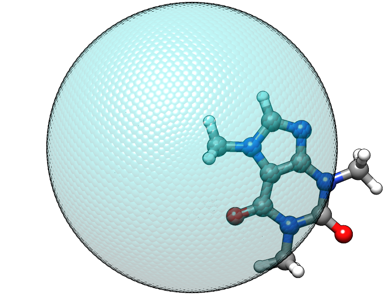
The sphere used to construct the potential is represented by the transparent teal dots placed on a fine Lebedev grid. Visual inspection suggests that the potential is misplaced.
To cope with this we should put the center of mass of the caffeine molecule
at the origin, this can be done by adding the $cma instruction to the input
file, which shifts the coordinates with the center of mass and aligns
the molecule to its principal axes of inertia.
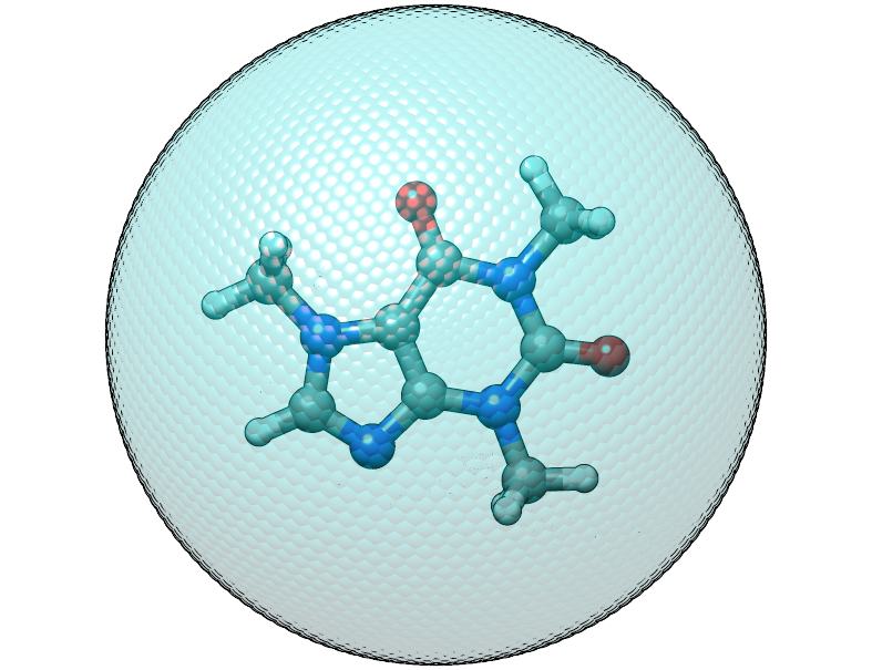
The caffeine molecule is now shifted correctly inside the potential. The confining energy, for the correctly placed potential is now 0 kcal/mol.
Note
The center point for all wall potentials is always placed at the origin, which cannot be changed with the currently available input options. Therefore, we resort to modifying our input coordinates here.
Different Potential Shapes
Currently two different potential shapes are implemented and can be
selected with the potential instruction.
The logfermi potential shape is given by the expression
where
kB is the Boltzmann constant,
T is formally the temperature but can be used to scale
the strength of the potential (adjustable by temp=<real>, within the $wall group),
β is the steepness of the potential (adjustable by beta=<real>),
RA are the cartesian coordinates of atom A,
O is the origin (0,0,0) and
Rsphere is the radius of the sphere used for confining.
The default potential shape is a simple polynomial to the power α
(adjustable by alpha=<int>).
The formula that is evaluated in the program is
The main (dis)advantage of this shape is that the radius of the sphere
is a relative quantity compared to the size of the molecule.
The auto generator of the sphere radius takes this into account,
by rescaling the largest distance in the molecule instead of adding
a constant shift.
A clear disadvantage of this potential shape it that the gradient does
not vanish inside the sphere and can compress a molecule artificially.
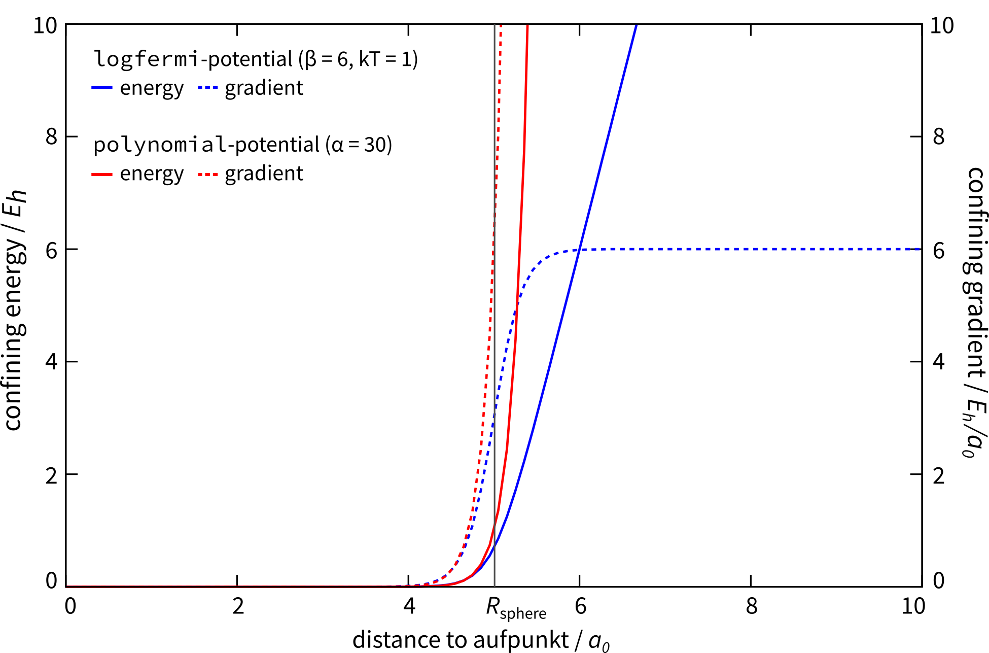
Available potential shapes with energy and gradient contribution.
Anisotropic Potentials
For some molecules an isotropic spherical cavity is not suitable for confinement, since the molecule might have a rod-like or oblate shape. Instead of sphere we can use an ellipsoid to construct an anisotropic cavity, there is no limitation for the potential shape since we use a simple rescaling to introduce anisotropy.
The input file for an anisotropic potential would look like
$wall
   potential=logfermi
   ellipsoid: 13.5,11.1,8.6,all # values in Bohr
$end
As for the isotropic one can use the auto keyword to replace any of the
the three radii with an automatically determined value.
The automatic determined value is the automatic isotropic sphere radius,
so letting all three values be autodetermined results in an isotropic potential.
As before, we have to deal with the issue that the center of mass of our caffeine molecule and the origin do not coincident, this time we use a Python interpreter with ASE support for this job
from ase.io import read, write
mol = read('caffeine.xyz')
mol.set_positions(mol.get_positions() - mol.get_center_of_mass())
write('caffeine_shifted.xyz', mol)
Finally we can check xtb with the new coordinates and the above input file and
we find that the confining energy is zero in the initial geometry.
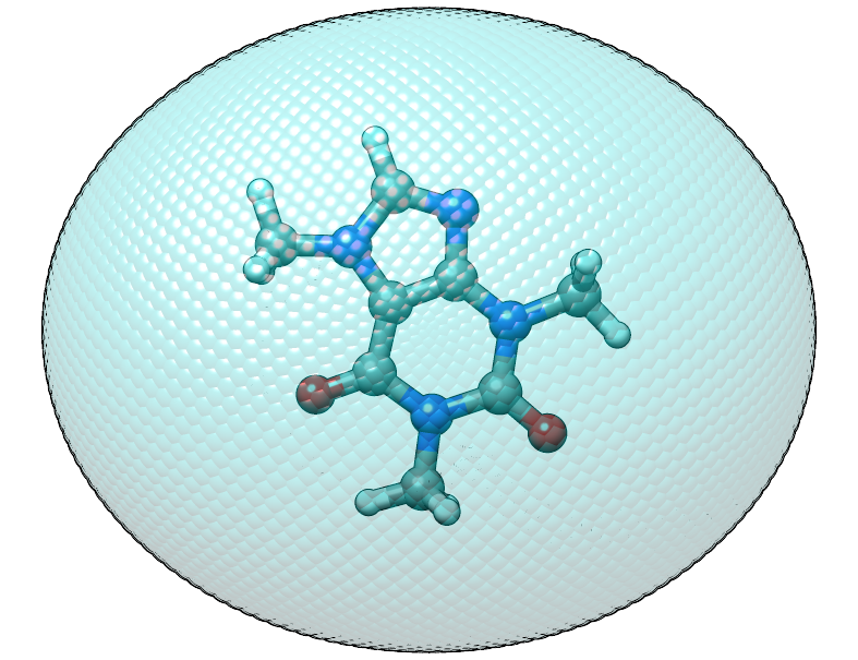
Shifted caffeine molecule in an anisotropic potential, note that the structure is not rotated this time.
Using Multiple Potentials
Since version 6.0 an arbitrary number of wall potentials is supported.
Similar to the constraint keywords one could create multiple wall potentials
by repeating sphere and/or ellipsoid instructions like
$wall
   potential=logfermi
   sphere: auto, all
   ellipsoid: 13.5,11.1,8.6,all # values in Bohr
$end
This could be used to confine different fragments in different sized spheres. The only restriction is that the potential shape is global.
Absolute Control
As I promised you can control almost everything, the xcontrol(7) man page
is a good starting point to get acquainted with the detailed input. This
poses the usual hindrance of actually reading the documentation
(since you are here, you are already above average, thumbs up).
A practical alternative is to just dump the complete internal settings of the program to an input file and start playing around with it. To do so, run
> xtb --input default.inp --define --copy coord
The file default.inp has not to be present when starting the program
in --copy mode, since the default.inp will be generated for you.
The --define flags makes sure that the program only checks your setup
and does not perform any calculation on the input coordinates.
Have a look at the first lines of default.inp:
$cmd xtb --input default.inp --define --copy coord
$date 2019/03/05 at 08:50:26.651
$chrg 0
$spin 0
...
This is actually the command you used in the first place to invoke the
program, next you find the timestamp when the program was started and
then system specific information about charge and spinstate of your system,
this is what I understand as a self-documenting program run.
$cmd and $date are cosmetic features and will never influence
any calculation if included in the detailed input, but I figured that
they might become handy if you look back into your calculations when
putting together the manuscript or taking over a project from your,
now graduated, fellow coworker.
The rest of the file represent every accessible variable documented
in the xcontrol(7) man page with its current setting, this should be
quite a lot. So lets focus say on the $wall group:
...
$wall
   potential=polynomial
   alpha=30
   beta=6.000000000000000
   temp=300.0000000000000
   autoscale=1.000000000000000
   axisshift=3.500000000000000
...
The default potential is a polynomial one, you want to change this to
the logfermi potential. alpha is only needed for the polynomial
potential, we use beta and temp in our potential.
The steepness of our potential can be adjusted by modifying the value
of beta, since our potential is multiplied with the thermal energy
we can scale it by increasing it temperature in temp.
autoscale is a factor the automatic determined sphere axes are
multiplied with, a default of 1.0 seems reasonable here, but sometimes
we need more space or want to squeeze everything a bit together.
We can also adjust the constant shift value used in the generation
of the automatic axes, but on a second thought this value might be
just fine, so we do not modify axisshift today.
This is an awful lot of information in a small block and quite essential
for your calculation using a confining potential, all details on this
can be found in xcontrol(7) man page at the group instruction
of interest.
Tip
If you are happy with all this setting you can just use this file as
your .xtbrc and place it somewhere in your XTBPATH.
Global Configuration File
The global configuration file called .xtbrc has to be around somewhere
in your XTBPATH so xtb is able to find it and uses the very same
syntax as the detailed input. Every instruction (key=value) you can
use in your detailed input file can be present in your global configuration
file. System specific instructions (key: value) will not work, of course.
To check which .xtbrc is read, start the program in verbose mode and
check the Calculation Setup section in the output.
Rules for Control
This section is intended to briefly explain the currently applied rules to parse the detailed input file.
Every instruction is started by a flag ($) and terminated by the next flag.
An instruction is only valid if the flag is in the first letter, the
instruction name is the rest of the register (line).
A valid instruction opens its block with its own options, every option
is a key-value pair. Invalid instructions are ignored without further warning.
There are two kind of instructions, logical and groups. Logical instructions toggle a specific operation and cannot contain a option block while group instructions only open the option block without any further actions.
Groups with the same name can occur multiple times and are merged before parsing.
There are two kind of options, key=value pairs set global variables and
can only be used once, they are locked at the first encounter of the key,
regardless of the value, in case an invalid value is given the default is used
as fallback and cannot be modified by subsequent options with the same key.
Options of the kind key: values,... can be present multiple times and
are handled differently depending on the context they are used in.
For example the atoms: instruction usually appends atoms to an list,
while distance: in $constrain applies a quadratic potential to
the atom pair specified.