Running QCxMS
The program runs in two modes: EI and CID. Both methods require three individual steps to create the final spectrum.
To obtain a QCxMS simulated mass spectrum, please follow this protocol:
Workflow of QCxMS
1. Setup
Prepare a file with the equilibrium structure of your desired molecule M. For the CID mode, the molecule has to be protonated. This can be done with the protonation tool of CREST.
Attention
The structure files can have all formats supported by the MCTC library , including coord and xyz file formats.
Prepare an input file called qcxms.in. The keywords can be found below and an example is given in in the examples folder. If no such file is prepared, [default] options are: run GFN2-xTB with 25 × the number of atoms in the molecule trajectories (
ntraj).
2. Preparing for Production Runs
Run
qcxmsfor the first time. This will generate the ground state (GS) trajectory from which information is taken for the production trajectories. After some steps for equilibration, the files trjM and qcxms.gs are generated.
Warning
This step already uses the QC method specified! As the correct sampling of the GS trajectory has no direct connection with the accuracy of the endresult, it is highly recommended to conduct the initial run with a low-cost method, e.g. GFN2-xTB [default] or GFN1-xTB.
Run
qcxmsfor the second time after the GS run is finished. If the qcxms.gs exists, this will create a TMPQCXMS folder and prepares the specifications for the parallel production.
3. Excecuting the Production Runs
If a computer cluster with a queing system is used, the
q-batchscript can be used for the execution of the parallel computations. This will initiate the production run withntrajtrajectories. For each trajectory this starts a single core calculation. If you want to run QCxMS locally, use thepqcxmsscript with-jnumber of parallel jobs and-tnumber of OMP threads:
pqcxms -j <integer> -t <integer> &
Attention
Look into the q-batch script, as it might need to be changed to match for your queing system!
The status of the QCxMS run can be checked by changing to the working directory and typing
getres, which will provide the tmpqcxms.res file (which can be plotted with PlotMS) and an output of the form:XXX runs done and written to tmpqcxms.res/out
The steps that are conducted in the production runs are displayed in the following figure. For details look into the qcxms.out file provided after the calculations are finished. For details on individual runs, look into the TMPQCXMS/TMP.X folder.
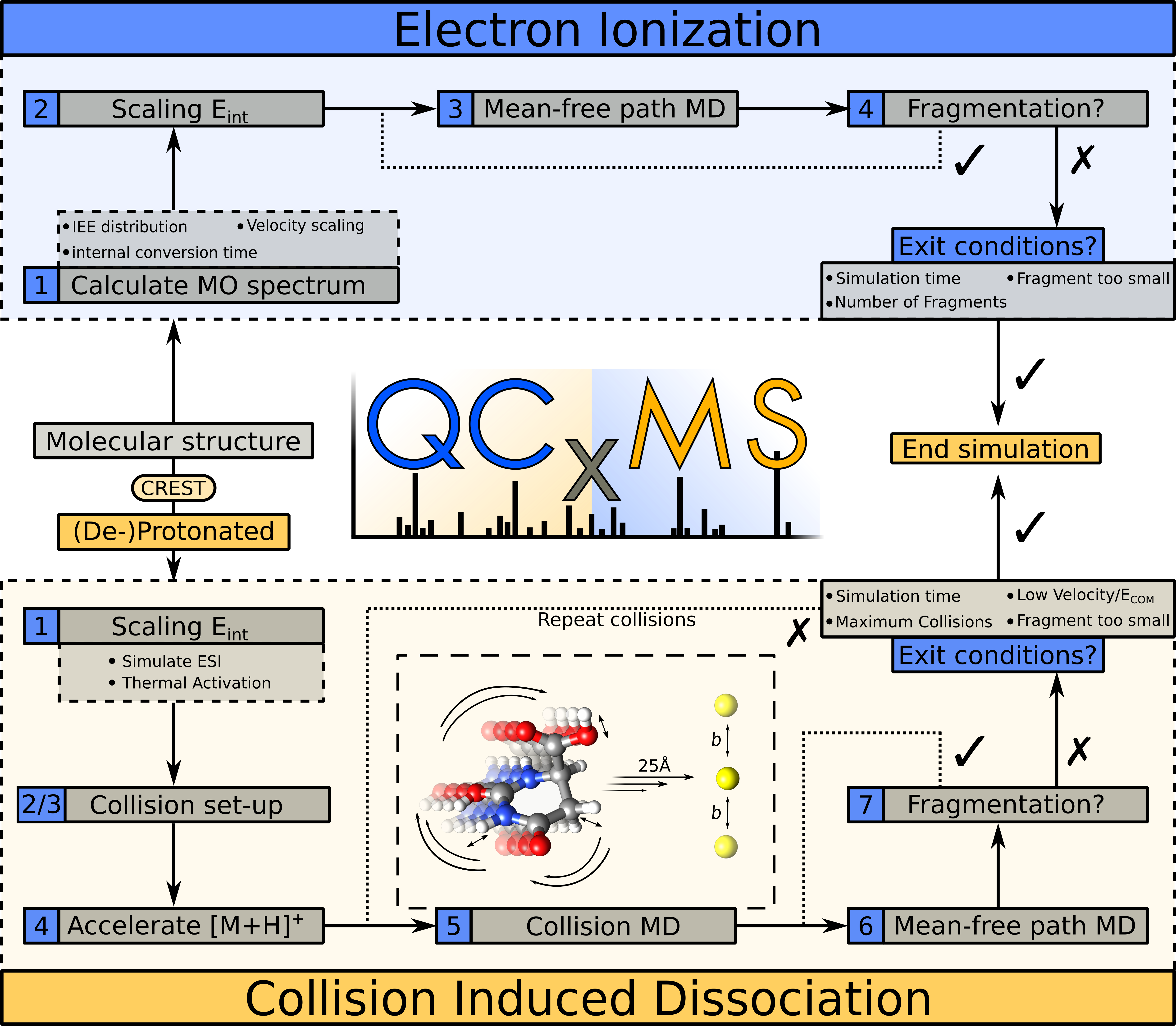
Steps during the production runs in the EI and CID modules. For details see: DOI: 10.1021/jasms.1c00098
As soon as the calculations are finished, the Visualization program can be used to analyse the resulting qcxms.res or qcxms_cid.res file and provides .agr (open with xmgrace), JCAMP-DX, and .csv files with the spectral data. If experimental data is put into the same folder in .csv format, a direct comparison to the computed spectrum is plottet into the .agr file and a matching score is provided. Run: plotms -i file.csv.
In each TMPQCXMS/TMP. file, a production run can be conducted by qcxms -p to test settings or take a look into the fragmentation processes in detail. Other qcxms_commandline options are provided below.
Input keywords in qcxms.in
If no input file is given, [default] settings are taken. This means an EI calculation is conducted. The general qcxms.in input file can be manipulated by providing <parameters> :
<Parameter> |
Specification |
Default |
Alt. settings |
|---|---|---|---|
<method> |
Mass Spec. Method |
ei |
cid, dea |
<program> |
QC Program |
xtb |
tmol, orca, mndo, dftb |
<method> |
QC Method |
xtb |
see: Input Details |
<qc settings> |
Basisset and/or Functional |
pbe0 sv(p) |
see: Input Details |
<ip method> |
Ionization Potential Method |
ip-xtb2 |
ip-xtb, ip-mndo, ip-tmol ip-orca/-orca5, ip-orca4 |
charge <integer> |
(neg.) Charge of M+ |
1 |
(-) <integer> |
ntraj <integer> |
Number of trajectories |
25 × no. of atoms |
<integer> |
tinit <real> |
Initial Temperature |
500 K |
<real> |
etemp <real> |
electronic Temperature |
5000 K |
<real> |
tmax <integer> |
Maximum MD time (sampling) |
5 ps |
<integer> |
tstep <real> |
MD time step |
0.5 fs |
<real> |
While xTB is set as [default] programm and method, it is not required to define it twice.
If ip-orca is chosen, ORCA 5.x is set as default. Chose ip-orca4 for version ORCA4.x.
The [default] charge is set to 1 for EI and CID computations. Negative charges can easily be set by providing charge -1, which switches the program automatically to the correct settings (i.e. DEA for negative charged EI). For multiple charges, e.g. set charge 2.
Attention
For EI, only 1 and -1 are considered. It is not possible to compute multiple charges with EI or DEA!
EI method specific keywords
<Parameter> |
Specification |
Default |
Alt. settings |
<mo method> |
Molecular Orbital |
mo-xtb |
mo-orca |
eimp0 <real> |
Electron-beam impact energy |
70 eV |
<real> |
eimpw <real> |
Impact energy distribution |
0.1 eV |
<real> |
ieeatm <real> |
Impact excess energy (IEE) per atom |
0.6 eV/atom |
<real> |
poisson or gauss (<real> <real>) |
IEE distribution type |
poisson |
<real> |
maxsec <integer> |
no. of secondary fragmentation runs |
7 |
<integer> |
nfragexit <integer> |
max. fragments created in single MD |
3 |
<integer> |
upper <real> |
upper limit for IEE distribution |
0 |
<real> |
lower <real> |
lower limit for IEE distribution |
0 |
<real> |
Changing the ieeatm amd eimpw values can have a significant influence on the fragmentation behavior of the molecular ion. For larger structures, the degrees-of-freedom (DOF) can require a larger setting of the impact excess energy per atom (ieeatm), as the energy distributed per atom can be too low.
Increasing this value can require increasing the impact energy eimp0 as well. If the IEE distribution has to be manually set, use the keywords upper and lower for the limit of the distribution.
Note
Poisson/Gauss IEE distribution: Generated from the MO spectrum of the molecule. For low ionization energies and for large molecules, the Poisson distribution may sometimes not converge. Switch to the Gauss distribution by specifying the gauss keyword. Two parameters may be entered, which manipulate the shape of the distribution. Caution! Manipulating the IEE distribution can lead to unphysical spectra with either over- or under-fragmentation of the precursor ion.
CID method specific keywords
<Parameter> |
Specification |
Default |
Alt. settings |
<run-type> |
Run-type specifics |
fullauto |
collauto, temprun |
elab <real> |
Collision Energy E(LAB) |
40 eV |
<real> |
ecom <real> |
Collision Energy E(COM) |
– |
<real> |
eexact |
do not distribute E(LAB) |
off |
none |
iatom <string> |
Neutral gas atom |
ar |
he, ne, kr, xe, n2 |
esi or tscale <real> |
E(int) or Temp. scaling |
mol. size (auto) |
<real> |
noesi |
switch off E(int) scaling |
off |
none |
pgas <real> |
gas pressure (Pa) |
0.132 (=1mTorr) |
<real> |
lchamb <real> |
coll. cell length (m) |
0.25 (=25cm) |
<real> |
setcoll <integer> |
number of pgc and fgc |
10 (collauto) |
<integer> |
maxcoll <integer> |
number of pgc, no fgc |
10 (collauto) |
<integer> |
collsec <int> <int> <int> |
number of fragmentations |
0 0 0 |
<integer> |
dist <int> |
number of steps until coll |
minimum 10 steps |
<integer> |
The center-of-mass energy (ecom) is a mass reduced value, defined as:
with \(m_g\) the mass of the collision gas, \(m_p\) the precursor mass and \(E_{kin}\) the kinetic energy of the precursor
ion (i.e. elab). It can be used as help for generalizing the input energy independent from the molecular ion size.
Providing the ecom command with a <real> value will automatically switch to the center-of-mass energy frame.
General Activation run-type (explicit collisions)
This run-type was developed to calculate spectra without manually setting many parameters. It is the [default] run-type, but can be called with the
fullauto command. The most important settings are lchamb defines the collision chamber length (in meters) and pgas the collision
gas pressure (in Pascal). The temperature of the gas is set to 300 K. These three factors are important for the number of precursor-gas collisions
(pgc) and fragment-gas collisions (fgc). It is advised to set the collision energy elab somewhat higher than in the experiments, depending on
the molecular ion’s size.
Forced Activation run-type (explicit collisions)
This run-type is called as soon as setcoll, maxcoll or collsec are called. The number of colllisions can be set to a total number of
collisions (pgc + fgc -> setcoll) or only precursor-gas collisions (pgc -> maxcoll). With the collsec mode, the number of
fragmentations are set (50%, 35%, 15% of runs).
Thermal Activation run-type (implicit collisions)
Increasing the internal energy can be done either by scaling the targeted temperature (tscale <real>) or internal energy (esi <real>).
Other important keywords
tmax: MD time for the mean-free-path (mfp) simulation in the EI mode. In the CID mode, this sets the number of time steps for the simulation after fragmentation during internal energy scaling (implicit run type). For the explicit run type, the time for the collision MDs is fixed at 50 fs * number_of_atoms.
eexact: No variation of the input collision energy; the molecular ion will be accelerated for all production runs with the same energy.
esi: A MD prior to the collision simulation (explicit run-types) increases E(int) to the <real> value. If this is less than the internal energy of the initial system (e.g. through high initial temperature), the scaling will be skipped (no downwards scaling/cooling!). If nothing is set, the scaling is done automatically depending on the system size (both general and forced [default on]).
noesi: Switch off the automaticesiscaling (explicit run-types). In the thermal activation run-type, this step cannot be skipped, as this is the essential part of the run-type.
Misc keywords
isotope <atomnumber> <mass_isotope> <atomnumber> <mass_isotope> … |
Switches <atom> <mass> to simulate isotopes. (integer masses) |
iseed <integer> |
Random number seed [default: off] |
etemp <real> |
Electronic temperature of convergenc of MD [default: Auto] |
nfragexit <integer> |
Stop at <integer> simultaneously created fragments [default: 3] |
ecp / no-ecp |
Use ECPs / Do not use ECPs (ORCA /TMOL only!) |
grid <integer> |
Set the ORCA grid [default: 2] |
Input Details
QC Programs:
Keyword |
Program |
Specifics |
xtb |
xTB |
built-in GFN1-xTB Hamiltonian |
xtb2 |
xTB |
built-in GFN2-xTB Hamiltonian |
tmol |
TURBOMOLE |
The ridft and rdgrad programs are called.distribution type |
orca orca5 orca4 |
ORCA ORCA ORCA |
QC program package version 5.0 (and higher) [default] QC program package version 5.0 (and higher) [default] QC program package version 4.0 (and higher) |
mndo |
MNDO99 |
semiempirical QC program available from Walter Thiel |
dftb |
DFTB+ |
semiempirical tight-binding QC program free for academic use |
SQM Programs:
The GFN1- and GFN2-xTB methods are available without any third-party software. All other semi-empirical quantum mechanical (SQM) methods have to be explicitly called with their corresponding program:
Keyword |
SQM Method |
Program |
Specifics |
xtb |
GFN1-xTB |
QCxMs |
D3-dispersion |
xtb2 |
GFN2-xTB |
QCxMS |
D4-dispersion |
om2 |
OM2-D3 |
MNDO99 |
D3-dispersion |
om3 |
OM3-D3 |
MNDO99 |
D3-dispersion |
am1 |
AM1-D3 |
MOPAC |
D3-dispersion |
pm3 |
PM3-D3 |
MOPAC |
D3-dispersion |
pm6 |
PM6-DH2 |
MOPAC |
D2-dispersion + h-bond |
dftb |
DFTB3-D3 |
DFTB+ |
D3-dispersion |
To decide which method should be used, it is recommended to read the original publication first! For using GFN1-xTB and GFN2-xTB with QCxMS, refer to the publications 4,5.
Note
The usage of AM1 or PM3/PM6 are not recommended, due to their bad performances!
Available Functionals in ORCA/TURBOMOLE:
Keyword |
Method |
DFT type |
Availability |
pbe |
PBE-D3BJ |
GGA |
ORCA / TURBOMOLE |
pbe0 |
PBE0-D3BJ |
global hybrid |
ORCA / TURBOMOLE |
pbeh3c |
PBEh3-c |
global hybrid |
ORCA / TURBOMOLE |
revpbe |
REVPBE-D3BJ |
GGA |
ORCA |
blyp |
BLYP-D3BJ |
GGA |
ORCA / TURBOMOLE |
b3lyp |
B3LYP-D3BJ |
global hybrid |
ORCA / TURBOMOLE |
tpss |
TPSS-D3BJ |
meta-GGA |
ORCA / TURBOMOLE |
b97d |
B97-D3BJ |
GGA |
ORCA / TURBOMOLE |
bp86 |
BP86-D3BJ |
GGA |
ORCA / TURBOMOLE |
b3pw91 |
B3PW91-D3BJ |
global hybrid |
ORCA |
m062x |
M062X |
meta-GGA global hybrid |
ORCA / TURBOMOLE |
pw6b95 |
PW6B95-D3BJ |
meta-GGA global hybrid |
ORCA / TURBOMOLE |
Available Basissets in ORCA/TURBOMOLE:
Keyword |
Basisset type |
Specification |
Availability |
sv |
double \(\zeta\) |
Split-valence (SV) |
ORCA / TURBOMOLE |
svx |
double \(\zeta\) + pol. |
SV + pol. func. on O,N |
ORCA |
sv(p) |
double \(\zeta\) + pol. |
SV + pol. func. on all except H |
ORCA / TURBOMOLE |
svp |
double \(\zeta\) + pol. |
SV + pol. func. on all |
ORCA / TURBOMOLE |
tzvp |
triple \(\zeta\) + pol. |
TZ + pol. func. on all |
ORCA / TURBOMOLE |
qzvp |
quad. \(\zeta\) + pol. |
QZ + pol. func. on all |
ORCA / TURBOMOLE |
def2-sv(p) |
double \(\zeta\) + pol. |
SV + pol. func. on all except H |
ORCA / TURBOMOLE |
def2-svp |
double \(\zeta\) + pol. |
SV + pol. func. on all |
ORCA / TURBOMOLE |
def2-svpd |
double \(\zeta\) + pol. + diff. |
SV + pol. and diff. func. on all |
TURBOMOLE |
def2-tzvp |
triple \(\zeta\) + pol. |
TZ + pol. func. on all |
ORCA |
def2-tzvpd |
triple \(\zeta\) + pol. + diff. |
TZ + pol. and diff. func. on all |
TURBOMOLE |
def2-qzvp |
quad. \(\zeta\) + pol. |
QZ + pol. func. on all |
ORCA / TURBOMOLE |
ma-def2-svp |
double \(\zeta\) + pol. |
min. aug. SV + pol. func. on all |
ORCA |
ma-def2-tzvp |
triple \(\zeta\) + pol. |
min. aug. TZ + pol. func. on all |
ORCA |
ma-def2-tzvpp |
triple \(\zeta\) + pol. + pol. |
min. aug. TZ + 2x pol. func. on all |
ORCA |
ma-def2-qzvp |
quad. \(\zeta\) + pol. |
min. aug. QZ + pol. func. on all |
ORCA |
Command line Options
- -c / –check
check IEE but do nothing (requires ground state trajectory). Writes IEE distribution in file eimp.dat.
- -p / –prod
production (fragmentation) mode. Possible in any existing TMPQCXMS/TMP.XXX directory.
- -eonly
use the requested QC (as specified in qcxms.in) and do a single-point energy.
- -e0
same as above, charge = 0
- -e1
same as above, charge = 1
- -qcp <string> / -qcpath <string>
<string> = path to the QC code. /usr/local/bin is the [default].
- -unity
enforces uniform velocity scaling during the vibrational heating phase (in EI mode only)
- -v / –verbose
provide more information on the starting settings.