ONIOM
This guide is aimed to give a general overview of the ONIOM implementation within the xtb program package.
Note
This feature is only present in version 6.6 and newer or in the current bleeding-edge version.
General description
The ONIOM scheme is a multiscale calculation approach used to treat large molecular systems efficiently. A detailed review of the ONIOM scheme and its possible applications can be found at: Chung2015.
The total two-layer ONIOM energy is defined as
where \(E_{whole, low}\) and \(E_{model, low}\) terms are the single-point energies calculated at a low-level of theory of the whole system and a specific system cutoff (called henceforward ‘inner region’). \(E_{model, high}\) denotes the single-point energy of the inner region at a higher level of theory. The idea is to combine the different theory levels in a subtractive manner to compromise accuracy and speed.
Input
To perform an ONIOM calculation with xtb the --oniom option is used. The inner region has to be defined by providing the atom numbers contained in it and two calculation methods (high:low) can be chosen. The ONIOM calculation is then invoked by callinig:
> xtb <geometry_file> --oniom [high]:[low] [inner_region]
Note
If high:low are not provided, the gfn2:gfnff combination is used.
Methods
gfnff, gfn1, gfn2
These methods are available in the xtb and can be utilized both as high and low-level approaches in the ONIOM framework.
Important
The ONIOM routine includes but is not limited to the xtb functionality. To expand the range of the available methods, the external ORCA and TURBOMOLE software packages can be employed. This is done by the addition of the corresponding binary path in the environment variable $PATH.
The best way to configure the external settings for the xtb run is to use xcontrol instructions.
orca
If ORCA should be employed, an orca input has to be provided to run calculations. An additional instruction file like xcontrol allows to specify the user-supplied orca input by adding the follwing lines:
$external
   orca input file=<filename>
or to provide only calculation method:
$external
   orca input string=<method>
If no input is specified, xtb writes an orca input with the default settings (B97-3c).
turbomole
Turbomole also uses its format to perform calculations, defined by the control file.
Initially, the xtb searches for the control file in the user’s calculation directory, and if no file is present, writes it with some default settings (B97-3c).
Note
Currently, it is possible to use ORCA/TURBOMOLE only as the high level embedding.
Inner region
To perform the ONIOM calculations with xtb one has to specify the inner_region_cutoff which is provided either directly as comma-separated indices (“1,3-5,9,10”), or via a file with the same content (or each index on a separate line).
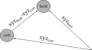
If covalent bonds are cut between the inner region and the rest of the system, ONIOM handles the resulting boundary through Hydrogen Linked Atoms (LAs):
The positions for LAs are determined by the positions of the cleaved atoms:
where \([xyz]_{con}\) and \([xyz]_{host}\) are coordinates of connector atom (stays in the inner region) and host atom (replaced by LA), \(k\) is a fixed scaling factor.
To distinguish between different bonds the topology information from the low level method is used.
Warning
It is strongly recommended to cut only single bonds. When using the GFN-FF as a low-level method, one has to be very careful with the inner region specification. The topology data of the GFN-FF does not allow for an accurate distinction between single and higher-order bonds.
Functionality
flags
- --chrg ‘int:int’:
extension of the classical
--chrgflag, allows to specify charges for inner region and whole molecule as inner_region_charge:system_charge. If only one value is given, it is used as system_charge, and thextbwill determine the inner_region_charge automatically.
Note
If inner_region_charge is specified in the external input format file(*.inp or control), one has to provide the same charge to the xtb as:
> xtb <geometry_file> --oniom <orca/turbomole>:<xtb> <inner_region> --chrg <inner_region_charge>:<system_charge>
- --uhf ‘int:int’:
extension of the classical
--uhfflag, allows to specify unpaired electrons for inner region and whole molecule as inner_region_uhf:system_uhf. If only one value is given, it is used as system_uhf, and the inner_region_uhf automatically.
Note
If inner_region_uhf is specified in the external input format file(*.inp or control), one has to provide the same charge to the xtb as:
> xtb <geometry_file> --oniom <orca/turbomole>:<xtb> <inner_region> --uhf <inner_region_uhf>:<system_uhf>
- --cut:
write the geometry of the specified inner region without performing any calculations. Note that hydrogen-linked atoms are not present, due to the absence of the Wiberg bond orders. In addition, this procedure can be used to test the abovementioned automatic inner region charge determination.
- --ceasefiles:
extension of the original flag, with instructions for the
xtbto delete all external files fromORCA/TURBOMOLE(except for*.inpandcontrolfiles)
xcontrol
In addition to the above-mentioned xcontrol instructions deeper control over the ONIOM routine is available via the $oniom group block.
- inner logs=[bool]
print high- and low-level optimization trajectory for the model system (
high.inner_region.logandlow.inner_region.log).- derived k=[bool]
k is a scaling factor for the LAs coordinates, which by default is constant. This instruction allows it to be dynamically assigned in dependence on the distance between the connector and host atoms.
- outer=[bool]
perform outer region saturation
- ignore topo=[bool]
bypass topology check when cutting bonds
- silent=[bool]
redirecting the output of the external programs into files.
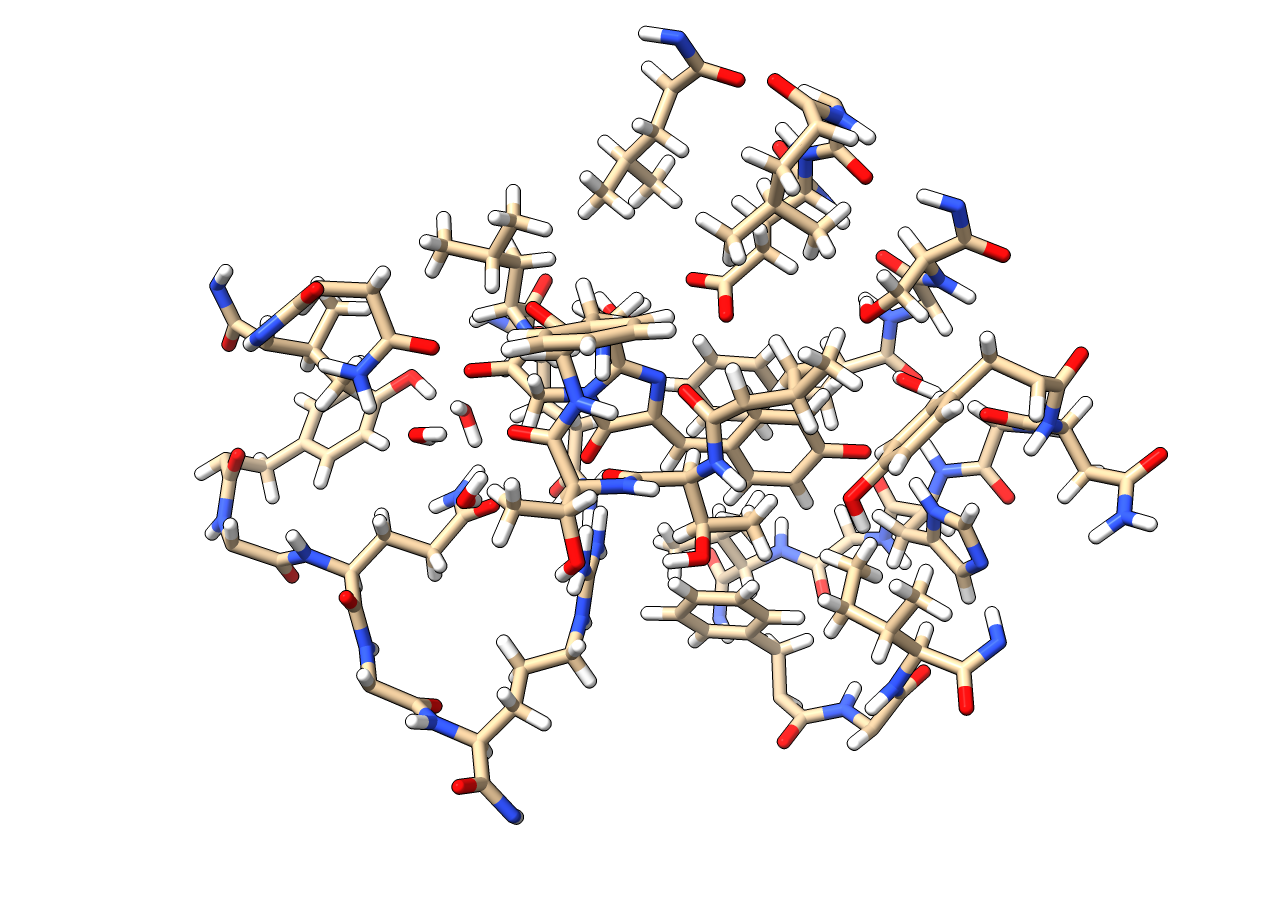
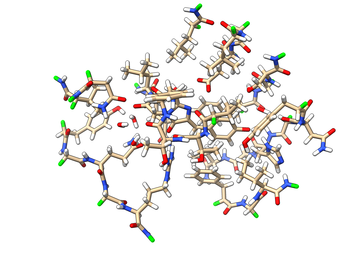
Example: S30L-23
As a showcase host-guest complex number 23 from S30L benchmark is chosen.
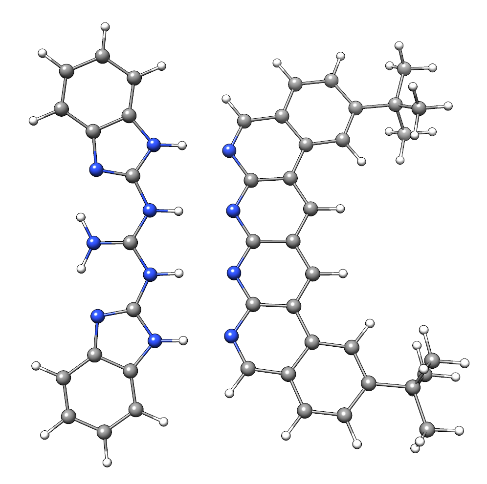
This system consists of 2 NCI-bound fragments: 1-62 and 63-98, the latter having +1 charge. To test the automatic charge identification routine:
> xtb input.xyz --oniom orca:gfn2 1-62 --chrg +1 --cut
98

C     0.7800079    6.8678780    5.5368969
C    -0.7524620   -6.8540954    5.5601280
C    -1.8617928   -4.6117174    5.6477616
C     0.6504601   -4.7941213    5.7959390
C     1.8907976    4.6261439    5.6192277
C    -0.6200120    4.8079116    5.7907513
C    -0.6206618   -5.3815968    5.1397097
C     0.6446437    5.3943761    5.1211667
C    -0.0083487   -0.0004324   -0.3233281
C     0.0816478    2.3154959   -0.3654186
C    -0.1026742   -2.3162587   -0.3590787
C    -0.2959652   -3.7207698    1.6988510
C     0.2900184    3.7253335    1.6873006
C    -0.1686909   -2.4104886    1.0817263
C     0.1605795    2.4132860    1.0744672
C     0.3073296    4.8471713    0.8195874
C    -0.3253307   -4.8444637    0.8338615
C     0.5276492    5.2249147    3.6051512
C    -0.5183472   -5.2156660    3.6222398
C    -0.0021327    0.0013275    1.1173800
C    -0.3936683   -3.9343044    3.0790781
C     0.4013815    3.9420198    3.0659794
C     0.1802918    4.6204737   -0.5828574
C    -0.2109397   -4.6213534   -0.5702540
C    -0.0947791   -1.2261541    1.7924088
C     0.0957022    1.2304873    1.7885605
C     0.5422958    6.3241699    2.7203124
C    -0.5452450   -6.3167433    2.7399789
C     0.4338755    6.1417501    1.3535797
C    -0.4505106   -6.1375070    1.3718405
N     0.0116094    1.1544899   -1.0315142
N    -0.0353108   -1.1570386   -1.0285348
N     0.0706724    3.4479104   -1.1540574
N    -0.1024078   -3.4505370   -1.1451747
H    -0.3766699   -3.0846938    3.7536939
H     0.3946574    3.0937118    3.7424387
H     0.6402108    7.3293416    3.1126263
H    -0.6416612   -7.3208096    3.1354374
H    -0.1065165   -1.2240152    2.8785113
H     0.1173973    1.2309738    2.8745222
H     0.4453140    6.9962771    0.6820918
H    -0.4716396   -6.9933848    0.7023244
H    -0.2080001   -5.4867763   -1.2347620
H     0.1678296    5.4843584   -1.2492380
H    -0.8214158   -6.9116715    6.6504902
H     0.8607175    6.9279102    6.6263141
H    -0.7372921    3.7424986    5.5676570
H     1.8239111    3.5571595    5.3925453
H    -1.7966759   -3.5433842    5.4175217
H     0.7662278   -3.7292650    5.5694116
H    -1.6551297   -7.3154982    5.1456164
H     0.1168724   -7.4441425    5.2509428
H     1.6777844    7.3288991    5.1115045
H    -0.0930120    7.4567246    5.2359300
H     2.8023074    5.0177240    5.1566686
H    -1.5202507    5.3298528    5.4510796
H    -2.7778232   -5.0041987    5.1950003
H     1.5472087   -5.3172918    5.4490088
H    -1.9411358   -4.7181202    6.7344847
H     0.5868113   -4.9026714    6.8834941
H    -0.5461631    4.9189786    6.8774015
H     1.9805730    4.7354338    6.7048538
C    -0.4488171    2.3665805   -4.6544687
C     0.4333778   -2.3789163   -4.6469142
C    -0.7917246    3.9457007   -6.0685007
C     0.7866666   -3.9602320   -6.0559302
C    -0.7915911    4.5371499   -4.7810591
C     0.7743565   -4.5501742   -4.7678612
N    -0.5769336    3.4887852   -3.8927405
N     0.5526308   -3.5004778   -3.8828746
N    -0.2162293    1.1365996   -4.0461490
N     0.1977398   -1.1476848   -4.0424055
C    -0.0069054   -0.0062888   -4.7519033
C     1.1701962   -6.6894301   -5.7142314
C    -1.1806924    6.6749532   -5.7335372
C    -1.1835769    6.0993249   -7.0168863
C     1.1847144   -6.1154023   -6.9982147
C     0.9956430   -4.7491407   -7.1892085
C    -0.9916821    4.7329808   -7.2045356
C    -0.9861523    5.9032143   -4.5891788
C     0.9658492   -5.9162071   -4.5726041
N    -0.0024966   -0.0075912   -6.0685751
N    -0.5736206    2.5723997   -5.9542885
N     0.5690957   -2.5866178   -5.9453246
H    -0.1946193    0.9005726   -6.5259354
H     0.1937665   -0.9163433   -6.5228612
H     0.1239780   -1.1213863   -3.0079656
H    -0.1481455    1.1124645   -3.0112686
H    -0.3819862    3.5198035   -2.8723700
H     0.3536032   -3.5294854   -2.8634564
H    -1.3407700    6.7384801   -7.8800928
H     1.3486405   -6.7558037   -7.8592332
H     1.3243264   -7.7589379   -5.6100014
H    -1.3357299    7.7446004   -5.6320230
H     1.0094379   -4.3072917   -8.1801901
H    -0.9964687    4.2898655   -8.1950479
H     0.9656238   -6.3638842   -3.5831368
H    -0.9956242    6.3520069   -3.6002631
           -------------------------------------------------
          |                Calculation Setup                |
           -------------------------------------------------

          program call               : xtb input.xyz --oniom orca:gfn2 1-62 --chrg +1 --cut
          hostname                   : albert
          coordinate file            : input.xyz
          omp threads                :                    16

   ID    Z sym.   atoms
    1    6 C      1-30, 63-68, 73-81
    2    7 N      31-34, 69-72, 82-84
    3    1 H      35-62, 85-98

  ... skip ...
  ------------------------------------------------------------------------
  |                        INNER REGION CHARGE =  0                      |
  ------------------------------------------------------------------------

normal termination of xtb
To start single-point calculation with the user-defined orca input file:
specify orca input and add its name in the xcontrol file:
   ! r2SCAN-3c
   ! engrad
   * xyzfile 0 1 some.xyz
$external
   orca input file=orca.inp
$end
Please use the engrad keyword to allow xtb to read the ORCA output. The inner region is automatically written in the some.xyz file.
start
xtbrun:
> xtb input.xyz --oniom orca:gfn2 1-62 --chrg +1 --input xcontrol
The final xtb output for the given example is divided into 3 parts with the ONIOM results printed in the property printout section:
   ------------------------------------------------------------------------

        Singlepoint calculation of whole system with low-level method

   ------------------------------------------------------------------------

   ... skip ...

   ------------------------------------------------------------------------

        Singlepoint calculation of inner region with low-level method

   ------------------------------------------------------------------------

   ... skip ...

   ------------------------------------------------------------------------

        Singlepoint calculation of inner region with high-level method

   ------------------------------------------------------------------------

   ... skip ...

             -------------------------------------------------
            |                Property Printout                |
             -------------------------------------------------

              -------------------------------------------------
             | TOTAL ENERGY            -1438.298999659396 Eh   |
             | GRADIENT NORM               0.045824034529 Eh/α |
              -------------------------------------------------